Modeling Apple's iPhone Camera
Using COMSOL's Ray Tracing Module
September 1, 2025
I have been using COMSOL Multiphysics since early 2017, and the Rayoptics module has always fascinated me. It interests me in large part because it produces these magnificent depictions of light rays, but also because it can be highly helpful in modeling misalignment in optical cavities. I have also been using cameras and been interested in photography since 2014. I thought it would be fun to merge these two aspects of my life and model the camera I use most often: the Apple iPhone camera.
To do this, I had to find a detailed description of an iPhone camera. Apple does not publish its camera lens configurations, so I had to dig into some patents to find one. That is when I saw the patent: "Wide field of view five element lens system". While the patent does not specify which iPhone it is incorporated into, the specs (F≈2.4 mm, F/2.0) and the year of the patent closely match those of the iPhone 11's front-facing camera, which has been tweaked and updated since. I bought an iPhone 11 Plus in 2019 when it was released, and figured this would be a good place to start. I can't be sure that this is an exact camera in the iPhone 11; in fact, it is almost certainly not identical to it, but it is certainly close, and more likely than not the inspiration for the final production camera. The final design used in the iPhone 11's front-facing camera is slightly different, with an aperture of F/2.2 and a focal length of 2.71 mm. This means that the production camera is somewhat worse than the ideal case presented in the patent.
A five-level lens system is relatively standard in cell phone cameras, as there isn't much room to include more lens elements. A 5-lens system is even used in COMSOL's own example compact camera. This makes it relatively simple to model. From the patent, I decided to model the lens system 710 configuration shown in Figure 7A, which has a 95° FOV and has its example values in Tables 1 through 3 in the patent. The hardest part of this was building the lens system. The values for curvature and aspheric curvature can be found in the table; however, values such as the actual diameter of the lenses had to be measured from Figure 7A. I broke these up into three Parameter files for COMSOL and imported them with an imaging plane and a stop to create the geometry shown below.
After creating the geometry and setting the material properties, which is only the index of refraction ($n_d$), I was finally able to set up the mesh and simulate. Interestingly, COMSOL does not allow the use of the Abbe number, which represents how different wavelengths of light refract due to the material. I decided to model the Abbe number by making the index of refraction a function of wavelength using Cauchy's equation, which allowed me to model dispersion. You can follow this process by hand, or you can use my Cauchy dispersion calculator.
Since the Abbe number can be expressed as
$$V_d=\frac{n_d-1}{n_f-n_c}.$$
With $n_d$ and $V_d$ given in the patent and referenced at the d-line 587.6 nm, I can solve for $n_f-n_c$. Let $\Delta=(n_d-1)/V_d$. Rather than assuming symmetry around $n_d$, I reconstruct $n_F$ and $n_C$ using the $1/\lambda^2$ weighting consistent with Cauchy. Define $x=1/\lambda^2$ and
$$t=\frac{x_d-x_C}{x_F-x_C},$$
where the three reference wavelengths are,
$$\lambda_F=486.1\text{ nm,}$$
$$\lambda_d=587.6\text{ nm,}$$
$$\lambda_C=656.3\text{ nm.}$$
Then we can see that
$$n_C=n_d-t\,\Delta,$$
$$n_F=n_d+(1-t)\,\Delta.$$
This gives three points:
- $n_F$ at $\lambda_F$
- $n_d$ at $\lambda_d$
- $n_C$ at $\lambda_C$
Next, I can fit the three values to Cauchy's equation,
$$n(\lambda)=A+\frac{B}{\lambda^2}+\frac{C}{\lambda^4}+...$$
where $\lambda$ is expressed in $\mu$m. The equation can be extended, but we will limit its order by only using the first three coefficients. This provides an expression for the index of refraction that depends on wavelength, enabling us to examine the dispersion of the lenses and their corresponding impact. In reality, I performed the above procedure three times, once for each index of refraction. With the geometry and materials fully defined, I could move on to the mesh.
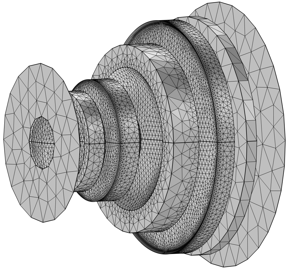
The mesh I used, shown above, employs a free triangular mesh for the optic faces, where I require the most precision, a physics-defined mesh, and a free tetrahedral mesh everywhere else. This mesh could be improved, but for this application, it is not overly fine and certainly works well enough.
Next, I set up the study, which consists of six sets of parallel rays entering the lens at varying angles, ranging from 0° to 45°. This stops just short of the 95° FOV claimed in the patent. Below, you can see the rays entering at different angles and being focused on various points on the sensor. If you are new to this type of optics, remember that the angle of light entering the lens corresponds to the location of the image. Since the light rays are parallel, this means the object is infinitely far away. This type of simulation is similar to taking a photograph of stars in the night sky.

The image above shows the light coming from different angles, focusing on various points on the sensor, which is indicated by the black line on the right side of the picture. This 2D model provides a clear view of what is happening inside the camera. One point of note at this point is that all the blue rays focus to a single point on the sensor at 0°, while the light coming in at 45° (the dark red) appears to be slightly out of focus. This probably indicates that my values for some of the lens curvature might be slightly off; Although I am very impressed with how close I got with just the values from the patent. Now that you have a good picture in your mind of what happens in 2D, I will show you the 3D image.
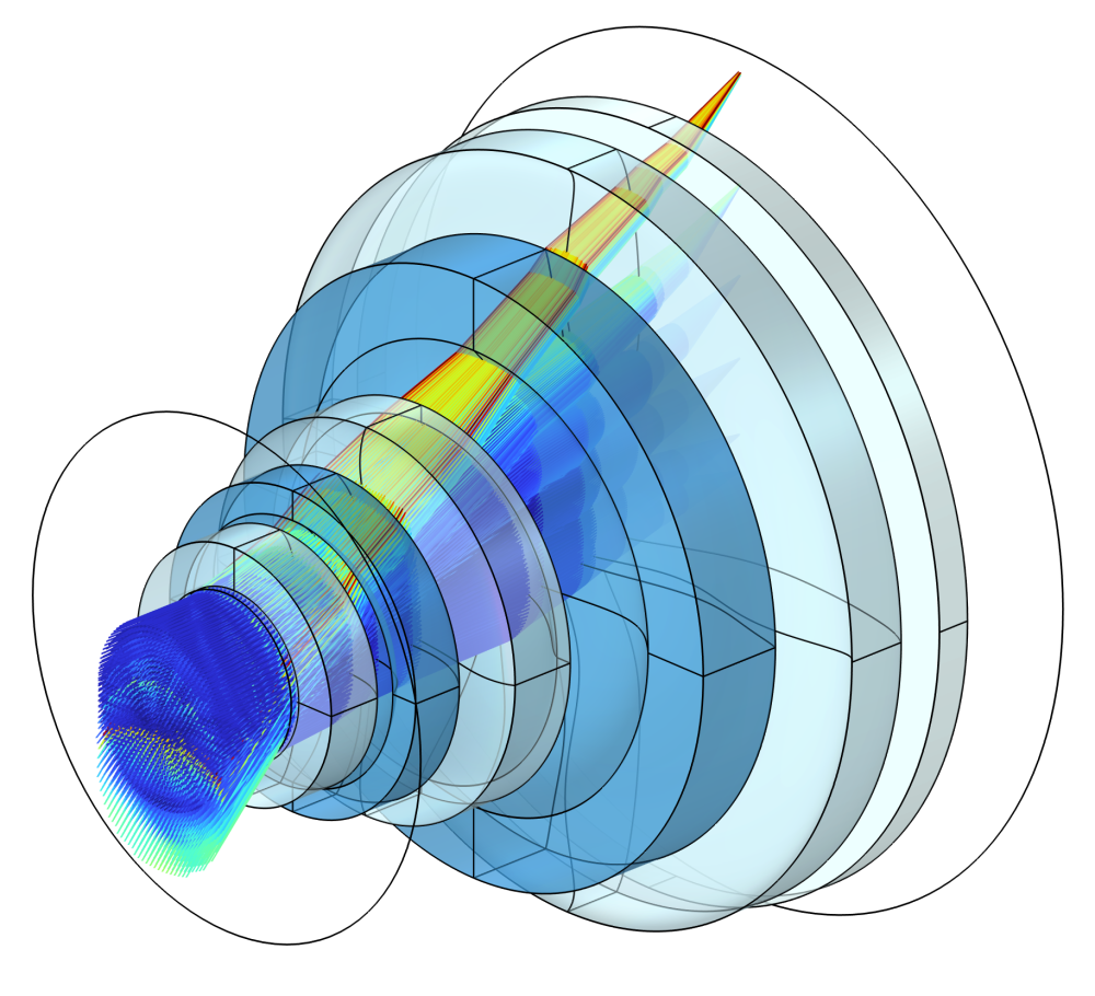
This looks similar to the 2D simulation but with many more rays. However, the same behavior is observed, where the rays converge to a point on the sensor, or at least ideally it is supposed to be focused to a point. We can map where all of these rays intersect the sensor plane and get a good sense of how well the camera performs.
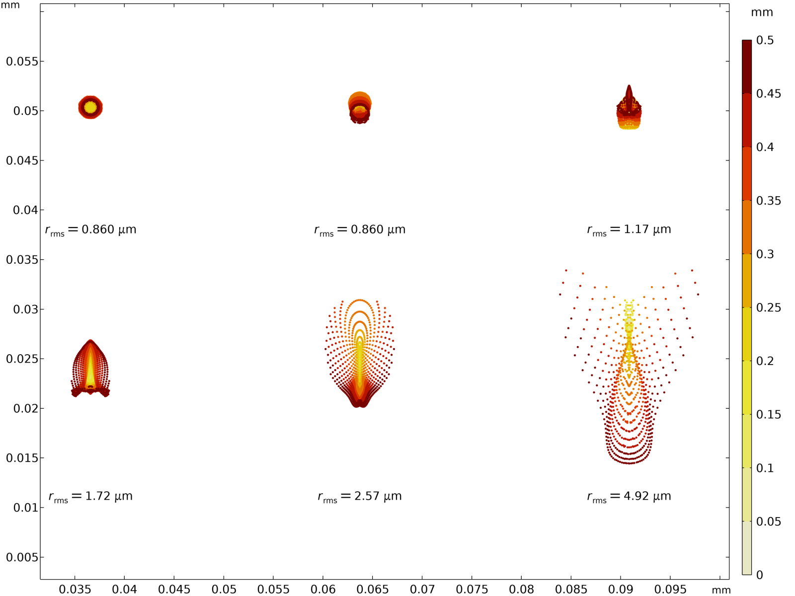
Above is the spot diagram, which shows the spread of points where each set of rays intersects with the focal plane. This theoretically lets you find the best focal plane by minimizing the RMS of the spread of points. It also illustrates an interesting, although not surprising, fact that photographers will already be familiar with: The center of the lens is the sharpest. The spot at the top left, which represents the rays at 0°, is perfectly radially symmetric and has the lowest RMS. To achieve the lowest RMS over all the angles, I actually had to move the sensor closer by 1%. Since the iPhone 11 has a pixel size of 1.4 $\mu$m, a tiny point of light can be resolved at the center of the lens, given my numbers for the lens prescription are correct. However, at the edges, the image may be slightly out of focus as the RMS value of 4.92 $\mu$m is larger than the pixel size.
I was hoping to find how different wavelengths of light would change how the image looked, but with the excellent engineering of this lens, the movement of the spots is only affected by 0.01 $\mu$m. On the scale of the 1.4 $\mu$m pixel size, this is non-existent. Since this is a relatively wide lens, minimal chromatic aberration is expected. Teephoto lenses typically show much greater chromatic aberration. I will have to try a different lens. I am already starting to model the Canon 70-200 mm f/4.0 lens that I have used since 2014.
One of the models I will be creating is the new Apple patent, "Camera modules with micro-scale optically absorptive gratings," which details a method for utilizing absorptive gratings to minimize the impact of lens flare. I think creating an absorptive element to target these bright lens flares is a fascinating idea.

